Quickstart

This tutorial provides a brief overview over the basic functionality of this package.

Matplotlib is imported for visualization

import matplotlib.pyplot as plt

Network generation

The layered model can be imported form the connectome.model package

from connectome.model import LL

The parameters of a model can be pre-defined

ll = LL(nr_neurons=2000, inh_ratio=.1,
        p_exc=.2, p_inh=.5, reciprocity_exc=.2)
ll

<LL nr_neurons=2000, p_exc=0.2, reciprocity_exc=0.2, inh_ratio=0.1, p_inh=0.5, nr_exc_subpopulations=∅>

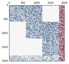
A network with three layers can now be generated

network = ll(nr_exc_subpopulations=3)
network

<Network nr_exc=1800, nr_inh=200>

and visualized

plt.matshow(network.adjacency_matrix, cmap="RdBu");

Similarly, a network with five layers is generated and visualized, executing

network_5 = ll(nr_exc_subpopulations=5)
plt.matshow(network_5.adjacency_matrix, cmap="RdBu");

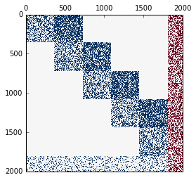
Please note that some parameters in the second call were still specified from the first call and therefore not passed again.

Network analysis

Summary statistics of a network are calculated with the help of the connectome.analysis package.

from connectome.analysis import RelativeCycleAnalysis

The number of cycles, relative to chance is computed with

cycle_analysis = RelativeCycleAnalysis(length=5)
cycle_analysis

<RelativeCycleAnalysis length=5, network=∅>

cycle_analysis(network=network)

{'relative_cycles_5': 0.19235267510727008}

The network contains less cycles of length 5 than expected by chance. A value above 1 indicates more cycles than expected by chance, a value below 1 indicates less cycles than expected by chance. The network’s reciprocity is calculated executing

from connectome.analysis import RelativeReciprocityEstimator
RelativeReciprocityEstimator(network=network)()

{'relative_reciprocity_ee': 1.0030832455128713,
 'relative_reciprocity_ei': 0.9991984266639169,
 'relative_reciprocity_ie': 0.999198426663917,
 'relative_reciprocity_ii': 0.9993940697569447}

The reciprocity obtained here, is close to the one expected from a pairwise random network.

Noise

Noise models are implemented in the connectome.noise package

from connectome.noise import RemoveAddNoiseAndSubsample

Random removal of half of the network’s connections with simultaneous reshuffling of 20% of the connections is simulated via

noise = RemoveAddNoiseAndSubsample(subsampling_fraction=.5, fraction_remove_and_add=.2)
noise

<RemoveAddNoiseAndSubsample subsampling_fraction=<InputChannel: subsampling_fraction=0.5>, network=<InputChannel: network=∅>, fraction_remove_and_add=<InputChannel: fraction_remove_and_add=0.2>>

noisy_network = noise(network=network)
noisy_network

<Network nr_exc=900, nr_inh=100>

This network has after perturbation only 1000 instead of 2000 neurons before.

plt.matshow(noisy_network.adjacency_matrix, cmap="RdBu");

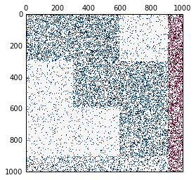
Additionally, connections on off-diagonal blocks appear; these were generated by the shuffling procedure. The number of cycles is also altered:

cycle_analysis(network=noisy_network)

{'relative_cycles_5': 0.68771057755341169}

The perturbed network has more cycles than the noise free version (0.192, see above).